SUMIFS is a function in Excel that allows you to sum values in a range that meet multiple criteria. Here's how you can use SUMIFS in Excel:
1. Select the cell where you want to display the sum of the values.
2. Type the formula "=SUMIFS(" into the cell.
3. Enter the range of cells that you want to sum in the first argument of the formula.
4. Enter the criteria range for the first criterion in the second argument of the formula.
5. Enter the criterion for the first criterion in the third argument of the formula.
6. Repeat steps 4-5 for each additional criterion.
7. Close the formula with a closing parenthesis ")" and press Enter.
Here's an example:
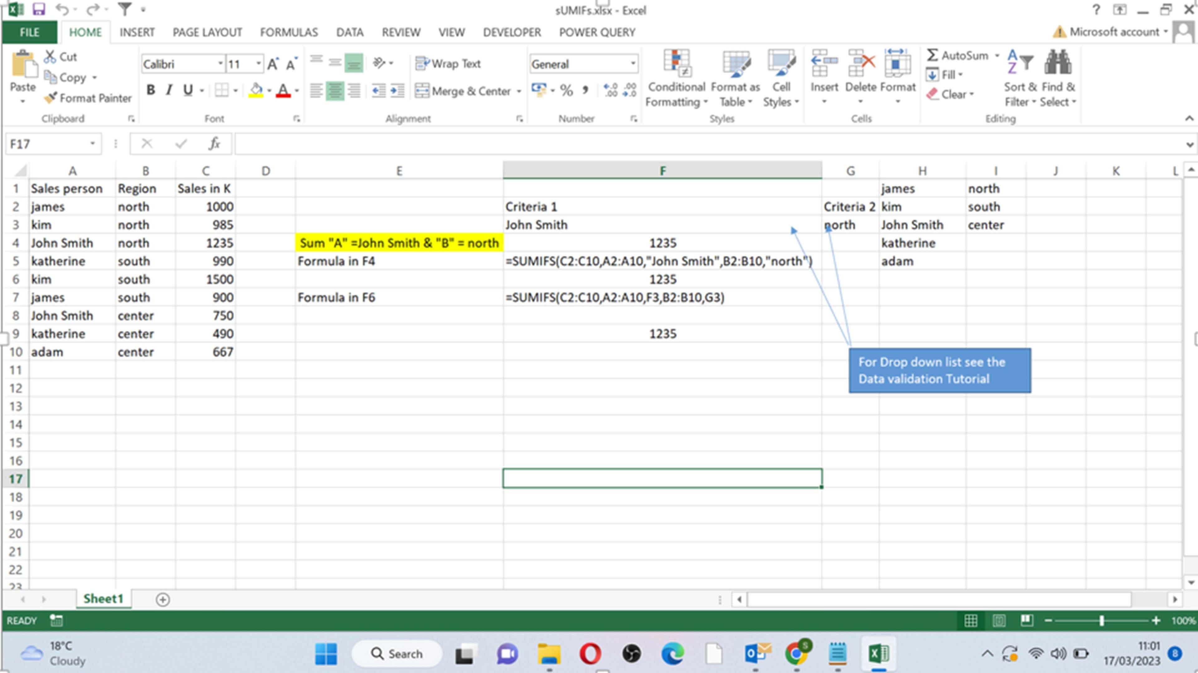
Let's say you have a table of sales data with columns for Salesperson, Region, and Sales. You want to find the total sales for a specific salesperson in a specific region. You would use the following formula:
You can Also insert the cell reference for criterias like
=SUMIFS(C2:C10, A2:A10, F3, B2:B10, G3)
In this formula, C2:C10 is the range of sales data that you want to sum, A2:A10 is the range of salesperson names, "F3" is the criterion for the first criterion, B2:B10 is the range of regions, and "G3" is the criterion for the second criterion.
Here's how you can use the SUMIFS function in Excel using the function wizard:
1. Select the cell where you want to display the sum of the values.
2. Click on the "fx" button next to the formula bar.
3. In the "Insert Function" dialog box, type "SUMIFS" in the search box or select it from the list of suggested functions.
4. Click on "OK".
5. In the "Function Arguments" dialog box, enter the range of cells that you want to sum in the "Sum_range" argument.
6. Enter the range of cells for the first criterion in the "Criteria_range1" argument.
7. Enter the criterion for the first criterion in the "Criteria1" argument.
Repeat steps 6-7 for each additional criterion.
Click on "OK" to close the dialog box and insert the formula into the cell.
The COUNTIF formula in Excel is used to count the number of cells in a range that meet a specific criteria. Here's how to use it:
1. First, select the cell where you want the result to appear.
2. Type the formula "=COUNTIF(" into the cell.
3. Select the range of cells you want to count.
4. Type a comma (",") after the range.
5. Enter the criteria you want to use for counting. This can be a number, text, or a cell reference to a value.
Close the formula with a ")".
Here's an example: If you want to count the number of cells in the range A1:A10 that contain the word "apple", the formula would be "=COUNTIF(A1:A10,"apple")".
You can also use operators such as "<" or ">" with COUNTIF. For example, if you want to count the number of cells in the range A1:A10 that are greater than 5, the formula would be "=COUNTIF(A1:A10,">5")". you can also give cell address for criteria like "=COUNTIF(A1:A10,">"& D5)" where D5 is the cell address. like this you can change the criteria in cell "D5".
To use the COUNTIF formula using the Function Wizard in Microsoft Excel, follow these steps:
1. Click on the cell where you want to display the result of the COUNTIF formula.
2. Click on the "Formulas" tab in the Excel ribbon menu.
3. Click on the "Insert Function" button. This will open the Function Wizard.
4. In the "Search for a function" box, type "COUNTIF" and press Enter. This will bring up the COUNTIF function in the list of available functions.
5. Click on the "OK" button to select the COUNTIF function.
6. In the Function Arguments dialog box, enter the range of cells you want to count in the "Range" field. You can do this by typing the cell range directly (e.g. A1:A10) or by clicking and dragging to select the cells.
Enter the criteria you want to use for counting in the "Criteria" field. This can be a number, text, or a cell reference to a value.
Click on the "OK" button to apply the COUNTIF formula and display the result in the selected cell.
Note that you can also access the Function Wizard by pressing the "fx" button next to the formula bar in Excel.
The VLOOKUP function in MS Excel is used to look up and retrieve data from a specific column of a table or range of cells. Here are the steps to use VLOOKUP in MS Excel:
1. First, select the cell where you want to place the result of the VLOOKUP function.
2. Type the formula "=VLOOKUP(" in the selected cell.
3. In the parentheses, enter the lookup value you want to search for.
4. After the lookup value, enter a comma and then the range of cells you want to search in. Make sure the first column of this range contains the lookup value.
5. Enter another comma and then the column number of the cell you want to retrieve data from.
6. Finally, close the parentheses and press Enter.
For example, suppose you have a table of student grades and you want to look up the grade of a student with the ID "123". The table is in cells A1:B5, with column A containing the student IDs and column B containing their grades. To use VLOOKUP to retrieve the grade of student 123, you would enter the formula "=VLOOKUP(123,A1:B5,2,FALSE)" in the cell where you want to display the result. This will search for the ID 123 in column A of the range A1:B5 and retrieve the corresponding grade from column B.
Note that the "FALSE" argument at the end of the formula indicates that you want an exact match for the lookup value. If you want an approximate match, you can use "TRUE" instead. You can also use 0 & 1 respectively.
The SUMIF formula in Excel is used to add up values that meet certain criteria. Here are the steps to use the SUMIF formula:
Open the Excel sheet where you want to use the SUMIF formula.
Select the cell where you want to display the result.
Type the following formula:
scss
=SUMIF(range,criteria,[sum_range])
Here, "range" refers to the range of cells that you want to check for the criteria, "criteria" refers to the condition that you want to apply, and "sum_range" refers to the range of cells that you want to add up (optional).
Replace the "range" and "criteria" values with the actual range and criteria that you want to use. For example, if you want to add up all the values in the range A1:A10 that are greater than 5, your formula would be:
if you want to give criteria then in the formula give the address of the cell as below e.g. in formula below the criteria will be in cell "E6".
less
=SUMIF(A1:A10,">5")
=SUMIF(A1:A10,">" &E6)
If you want to add up values in a different range than the range that you're checking for criteria, add that range as the third argument in the formula. For example, if you want to add up values in the range B1:B10, your formula would be:
less
=SUMIF(A1:A10,">5",B1:B10)
Press Enter to complete the formula. The result should be displayed in the selected cell.
That's it! You have now successfully used the SUMIF formula in Excel.
Alternatively, you can use the Function Wizard to help you build your SUMIF formula. Here's how:
Select the cell where you want the result to appear.
Click on the formula bar or fx bar at the top of the screen.
Type "=SUMIF(" followed by the range of cells you want to evaluate.
Click on the "fx" button next to the formula bar to open the Function Wizard.
In the Function Wizard, select the SUMIF function from the list of functions or type it in the search bar.
Follow the prompts to enter the criterion or condition you want to apply and the range of cells you want to sum.
Click OK to insert the formula into the formula bar and press Enter to calculate the result.
Remember to adjust the range of cells and criterion or condition to suit your specific needs.
Data validation is a feature in Microsoft Excel that allows you to control the type of data that can be entered into a cell or range of cells. Here are the steps to use data validation in Excel:
Select the cell or range of cells where you want to apply data validation.
Go to the Data tab in the Excel ribbon and click on the Data Validation button in the Data Tools group.
In the Data Validation dialog box, choose the type of validation rule you want to apply. The most common types of validation rules are:
Whole number: to allow only whole numbers for example we have validation between 1 & 1000 any value other than it will result in error.
Decimal: to allow only decimal numbers for example we have validation between 1.1 & 3.0 any value other than it will result in error.
List1: to allow only values from a specified list for example we have validation between Text1, Text2 & Text3 any Text other than it will result in error.
List2: to allow only values from a specified list for example we have validation between Cell K2 to K4 any Text other than contained in it will result in error.
the "Data Validation" feature can be used to create a dropdown list of options for a cell. Here's how to do it:
Select the cell or range of cells where you want the dropdown list to appear.
Go to the "Data" tab in the ribbon and click on "Data Validation" in the "Data Tools" group.
In the "Data Validation" dialog box, under the "Settings" tab, select "List" in the "Allow" drop-down menu.
In the "Source" field, enter the list of options you want to appear in the dropdown, separated by commas. For example: "Option 1, Option 2, Option 3".
You can also choose to show an error message or restrict input to only the items in the list by selecting the appropriate options under the "Error Alert" tab.
Click "OK" to close the dialog box and apply the validation to the selected cells.
Now, when you click on the cell or range of cells, a dropdown arrow will appear, allowing you to select one of the options from the list you created.
Date: to allow only date values within a specified range
Time: to allow only time values within a specified range
Once you have selected the validation rule, enter the required information. For example, if you choose the List option, you need to enter the list of allowed values in the Source box.
Optionally, you can also enter an error message that will be displayed if the user enters an invalid value. You can also set a warning message to appear if the user enters a value that is close to the limit.
Click on the OK button to apply the validation rule to the selected cells.
Now, when a user tries to enter data into the validated cells, Excel will check if the entered value meets the validation criteria. If the value is not allowed, Excel will display an error message and prompt the user to enter a valid value.
There are many basic formulas in Microsoft Excel that you can use to perform calculations and analysis on your data. Here are some of the most commonly used ones:
SUM: Adds up a range of numbers. The formula syntax is "=SUM(range)". & "=A1 + B1"
SUBTRACT: Devides one cell value from other. The formula syntax is "=A1-B1".
Devide: Devides one cell value with other. The formula syntax is "=A1/B1".
MULTIPLY: Multiplies one Cell value with Other. The formula syntax is "=A1*B1".
AVERAGE: Calculates the average of a range of numbers. The formula syntax is "=AVERAGE(range)".
MAX: Returns the largest value in a range of numbers. The formula syntax is "=MAX(range)".
MIN: Returns the smallest value in a range of numbers. The formula syntax is "=MIN(range)".
COUNT: Counts the number of cells in a range that contain numbers. The formula syntax is "=COUNT(range)".
IF: Tests a condition and returns one value if the condition is true and another value if the condition is false. The formula syntax is "=IF(condition, value_if_true, value_if_false)".
VLOOKUP: Searches for a value in the first column of a range and returns a value in the same row from a specified column. The formula syntax is "=VLOOKUP(lookup_value, table_array, col_index_num, [range_lookup])".
CONCATENATE: Joins two or more text strings into one string. The formula syntax is "=CONCATENATE(text1, [text2], [text3], ...)" or "=CONCATENATE(A1, B1, C1, ...)". assuming A1, B1 & C1 contain texts 1, 2 & 3.
LEFT: Extracts a specified number of characters from the beginning of a text string. The formula syntax is "=LEFT(text, num_chars)" or = "LEFT(A1, num_chars)" assuming A1 contains the text.
RIGHT: Extracts a specified number of characters from the end of a text string. The formula syntax is "=RIGHT(text, num_chars)". or = "RIGHT(A1, num_chars)" assuming A1 contains the text.
These are just a few examples of the many formulas available in Microsoft Excel. By mastering these basic formulas, you can perform a wide range of calculations and analysis on your data.
Getting Started: When you open Excel 2013, you'll see a blank worksheet with a grid of rows and columns. Each column is labeled with a letter and each row is labeled with a number. You can select a cell by clicking on it.
At the top of an Excel sheet, you will find several important elements:
Ribbon: The Ribbon is a horizontal bar that contains tabs, each with a collection of commands and functions. The tabs are Home, Insert, Page Layout, Formulas, Data, Review, and View. You can use these tabs to perform various tasks in Excel, such as formatting cells, inserting charts, and sorting data.
Quick Access Toolbar: The Quick Access Toolbar is a customizable toolbar that contains shortcuts to frequently used commands. By default, it contains commands like Save, Undo, and Redo, but you can add or remove commands as needed.
Name Box: The Name Box is a box located to the left of the Formula Bar that displays the cell address of the active cell. You can use the Name Box to quickly navigate to a specific cell by entering its cell address.
Formula Bar: The Formula Bar is a bar located above the worksheet that displays the contents of the active cell. You can use the Formula Bar to enter or edit formulas and functions.
Column and Row Headers: The column headers are the letters at the top of each column (A, B, C, etc.), and the row headers are the numbers at the left of each row (1, 2, 3, etc.). You can use the column and row headers to reference specific cells in your formulas and functions.
Overall, these elements at the top of an Excel sheet are important tools that you can use to navigate, format, and analyze your data.
In Excel, cells are labeled with a combination of letters and numbers. The letter represents the column and the number represents the row. For example, the cell in the top left corner of the worksheet is labeled A1.
Here are some ways cells are used in Excel:
Data Entry: You can enter text, numbers, dates, and formulas into cells. This data can be used for calculations, analysis, and visualization.
Calculation: Excel can perform calculations on the data entered in cells using formulas and functions. You can use basic arithmetic operators (+, -, *, /) or more advanced functions to perform calculations.
Formatting: You can format cells to change their appearance. This includes changing the font, font size, font color, background color, and alignment. Formatting can make your data easier to read and understand.
Conditional Formatting: Conditional formatting allows you to highlight cells that meet certain conditions. For example, you can highlight cells that contain a certain value or that are above or below a certain threshold.
Charts: Excel can create charts to help you visualize your data. You can select a range of cells and create a chart that shows the data in a graphical format. There are many types of charts to choose from, including bar charts, line charts, and pie charts.
Sorting and Filtering: Excel allows you to sort and filter data in cells. You can sort data by column to arrange it in ascending or descending order. You can also filter data to show only the data that meets certain criteria.
Overall, cells are the building blocks of Excel worksheets. By entering data into cells, formatting cells, and using formulas and functions, you can perform calculations, analyze data, and create visualizations to help you make informed decisions.
Entering Data: To enter data into a cell, simply click on the cell and start typing. You can enter text, numbers, dates, and formulas. To move to the next cell, press the Enter key.
AutoSum: AutoSum is a quick way to add up a range of cells. Select the cell where you want the total to appear, click on the AutoSum button, and Excel will automatically add up the cells above.
Functions: Excel has a variety of functions that you can use to perform calculations. To use a function, type "=" followed by the name of the function and the range of cells you want to include in the calculation. For example, "=SUM(A1:A5)" will add up the values in cells A1 through A5.
Printing: To print your worksheet, click on the File tab and select "Print." Here, you can choose the number of copies, the printer, and the page layout.
These are just a few of the basics of Excel 2013. As you become more comfortable with the program, you can explore more advanced features like conditional formatting, pivot tables, and macros.